
Data Analysis with Pandas: Unlocking the Power of Dataframe Operations

Key characteristics of a Pandas DataFrame:
-
Rows and Columns: DataFrames feature rows and columns, and each column may include a variety of data types (such as integers, floats, texts, etc.). A DataFrame can be thought of as a grouping of Series objects, where each column is a Series.
-
Flexibility: DataFrames are useful for processing a variety of datasets since they can contain heterogeneous data types within the same DataFrame.
-
Size Mutability: After a DataFrame is generated, you can add, remove, or change the rows and columns in it.
-
Labeling: Row and column labels in DataFrames allow you to access particular data items. Strings or integers are frequently used as row labels and column labels.
-
Data Operations: Pandas offers a variety of tools and methods for manipulating data, such as grouping, merging, filtering, and reshaping.
Common DataFrame operations in pandas:
-
Creating DataFrames — pd.DataFrame(data, columns): Creates a DataFrame from various data sources, such as lists, dictionaries, or other DataFrames.
-
Viewing Data:
-
df.head(n): Returns the first n rows of the DataFrame. -
df.tail(n): Returns the last n rows of the DataFrame. -
df.shape: Returns the dimensions (rows, columns) of the DataFrame. -
df.columns: Returns the column names. -
df.index: Returns the row index.
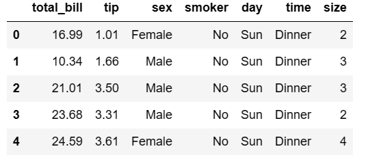
For example, let us consider a dataset “tips” to display the first 5 rows of the dataframe.
For which we have to import the pandas package and seaborn package where the tips dataset is available. The code follows like this
#import pandas and seaborn packages import seaborn as sns import pandas as pd #loading the dataset from the seaborn package into the tips dataframe tips = sns.load_dataset('tips') #calling the head function to return the first 5 rows first_5_rows = tips.head(5) #printing the rows first_5_rows
Output:
- Indexing and Selecting Data:
-
df[column_name]: Selects a single column. -
df[[col1, col2]]: Selects multiple columns. -
df.loc[row_label]: Selects a row by label. -
df.iloc[row_index]: Selects a row by integer index. -
df.loc[row_label, column_name]: Selects a specific cell by label. -
df.iloc[row_index, col_index]: Selects a specific cell by integer index. -
Boolean indexing: Allows you to select rows based on a condition, e.g., df[df['column'] > 5].
4. Filtering Data:
-
df.query(“condition”): Allows you to filter rows based on a query condition. -
df[df['column_name'].isin(values)]: Filters rows based on a list of values.
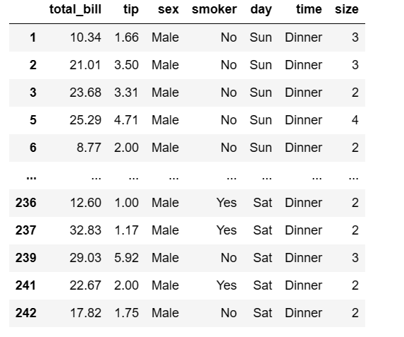
Let us consider an example using the tips dataset to filter and display only the male gender.
#create dataframe for only sex == male tips.loc[tips['sex'] == 'Male']
Output:
5. Sorting Data:
-
df.sort_values(by='column_name'): Sorts the DataFrame by a specific column. -
df.sort_values(by=['col1', 'col2']): Sorts by multiple columns. -
df.sort_index(): Sorts by the index.
6. Data Cleaning and Transformation:
-
df.drop(columns=['col1', 'col2']): Drops specified columns. -
df.rename(columns={'old_name': 'new_name'}): Renames columns. -
df.fillna(value): Fills missing values with a specified value. -
df.drop_duplicates(): Removes duplicate rows. -
df.apply(func): Applies a function to each element in the DataFrame.
Here is the code for forward filling which means filling missing values with the values from the previous row in the same column.
data.fillna(method = 'ffill', inplace = True )
Here, the 'inplace=True' indicated the in place parameter, when set to True, indicates that the operation should be performed on the DataFrame itself. If set to False, then the operation would return a new DataFrame leaving the original DataFrame unchanged.
7. Statistical Analysis:
-
df.describe(): Provides summary statistics for numeric columns. -
df.corr(): Computes the correlation matrix. -
df.cov(): Computes the covariance matrix.
8. Reshaping Data:
-
**
df.pivot(index='row_col', columns='col_col', values='value_col'): **Pivot table operation. -
df.melt(id_vars=['col1'], value_vars=['col2']): Melts a DataFrame.
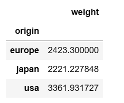
Let us consider an mpg dataset from the Seaborn package and create a pivot table to calculate the average weight of cars manufactured in each country.
import seaborn as sns import pandas as pd #loading the dataset from the package and storing it in a dataframe mpg = sns.load_dataset('mpg') #Create pivot table mpg.pivot_table(index='origin', values='weight', aggfunc='mean')
Output:
Pandas and Collaborating Libraries:
The strength of Pandas' DataFrame operations resides in its capacity to offer a flexible and effective framework for Python data manipulation and analysis.
While pandas is a potent tool for data manipulation and analysis, additional specialized libraries in the Python ecosystem supplement its strength. For instance:
-
NumPy is often used alongside pandas for efficient numerical operations on data.
-
Matplotlib and Seaborn are used for data visualization.
-
Scikit-learn is used for machine learning tasks.
-
Statsmodels is used for statistical modeling.
Hence, the choice of which library to use depends on the specific task at hand. Overall, pandas is a well-liked option for data manipulation and analysis in Python because of its combination of simplicity, adaptability, and performance.
In the world of data analysis, the pandas library and its indispensable tool, DataFrames, shine as the unsung heroes. These versatile structures offer a streamlined approach to data manipulation, enabling data professionals to efficiently clean, transform, and analyze data, regardless of its size or complexity. As we've explored in this blog, pandas provide a solid foundation for any data-driven project, fostering productivity and paving the way for deeper insights. Whether you're a seasoned data scientist or just beginning your journey, mastering pandas and its DataFrames is a crucial step towards unlocking the true potential of your data and elevating your data analysis game.